2d Collision Resolution

Most of the formulas we calculated in 3 dimensions should carry over into 2 dimensions, only with a few minor differences. The purpose of this post is to discuss those differences. With that in mind you should read and thoroughly understand the previous post on the full details of 3d collision resolution before reading this.

Computing Angular Inertia

The inertia tensor is now a scalar, and the orientation can be represented with a scalar value describing the rotation from its initial orientation. It still remains true that:

Formula 1:

Only , and are scalars now as well.

For cross products, things get a little weird. Our torque and impulsive torque formulas were as follows:

and

The cross product is defined only in 3 dimensions, but we can cheat a bit by briefly imagining the vectors and as living in 3D space and having a 0 z-component. The cross product, being normal to the 2 vectors will be in the z direction, but the z coordinate will still describe the appropriate, signed torque magnitude.

If we compute the cross product (let’s replace with for short:

One way we can extract the z component is to simply dot the vector with the vector. With this we can write our next 2D formula:

Formula 2:

Using the Formula 2 to substitute for in Formula 1, and integrating both sides over a time duration from to , we have:

Similarly as before, if we assume that for some constant  unit vector , by observing that cross products are distributive, and that dot products are also distributive, and since and are constants, we can factor out the left side and right side of the integral, so that we can integrate only over the time dependent values:

Now note the left hand integral is simply (which again, is a scalar), and the right hand integral is simply (the impulse as a scalar. So we can rewrite the above equation as:

And if we combine the unit vector and the scalar impulse into a single vector (in the direction of with with magnitude equal to then we have:

Formula 3: 

We can now expand out Formula 3 to yield Formula 4:

Formula 4:

Note, we could fairly easily come up with a fairly intuitive, geometric derivation of the torque Formula 2 without going into 3 dimensions. We could simply  take the normalized, 90 degree rotated vector to obtain the direction of the normal force, dotted this with the force vector and then multiplied by the torque arm length which would cause a canceling effect, resulting in:  which we could write as:

Formula 2.1:

Where is a 90 degree rotation matrix. Once again, we could take advantage of the dot product being distributive to pull out a time integral of force and arrive at a similar impulse formula:

Formula 3.1:

When we multiply this out we obtain Formula 4 anyway, it was just to show that both the 2D and “Mock 3D” approach agree.

Linearizing rotation

Again, there are two approaches we can take for this.

The first is to take the 3D approach. The impulse torque would be computed as a vector in the z axis, but the 2nd cross product that linearizes the velocity, and restores it to the xy plane.

The 3d formula we use is Formula 5.5 from our previous post:

(Formula 5.5 from previous post):

If we bite the bullet and manually expand out these two cross products, we obtain the following (we drop the 0 z-coordinate from the result):
Formula 5:

The second approach is via geometry.

If the vector P is rotating at an angular velocity then the speed of the tip of that vector is trivially: .

The (unit) direction of that motion will be the perpendicular vector resulting from a counter clockwise rotation, and then normalized, which we know to be:

.

Multiplying the speed times the direction gives us the velocity vector:

Which simplifies to:

Replacing with in Formula 4 (recalling that we can use quantities like and interchangeably):

Carrying out the multiplication we obtain Formula 5 once more:

Formula 5:

Now let’s see something magical. Recall that for resolving penetration in 3D we use the frictionless derivation of the inertia quantity, in which the impulse is treated as a scalar applied in the direction of the contact normal . In formula 5 we see the resulting delta in velocity as a result of an arbitrary 2d impulse vector (in particular, the delta in velocity as a result of rotation).
So if we replace with where is now a scalar, and substitute this in Formula 5 above we obtain:

Formula 6:

Now that we have the resulting linearized velocity, we must dot with the contact normal :

Computing the dot product:

Simplifying:

Formula 7:

Observe we have a perfect square! This produces the intuitive result that a positive impulse in the direction of the contact normal should always induce a rotation in the direction of the contact normal. After all, our moment of inertia is a scalar, so it will never redirect the motion in a weird way, it will only slow it.

We have effectively figured out the frictionless angular inertia quantity for a single rigid body in 2d (we remove the from the right side of Formula 7):

Formula 8: 

The linear inertia for a single rigid body is unchanged from before:

Formula 9:

By the same reasoning as before, accounting for reversed forces for body1, and the fact that we subtract the body1 velocities to obtain closing velocity, we reach the following inertia formula:

Formula 10: 

Now that we have new inertia formulas, we should be able to resolve the penetration in the exact same way as before. The only slight modification will be how we apply the calculated rotation.

Applying the rotation

First we recall equation 4, and again replace with where is a scalar.

As before, we determine how much time it takes to cross the angular move distance (not I use t’ instead of t only to agree with a previously used convention):

which gives:

therefore:

Note how the cancels and we obtain:

Formula 11:

Observe that this is merely a scalar, and so we can simply add it to the rotation scalar to apply it (no fancy quaternion functions needed).

Note this is the result for body0 but the result for body1 would be analogous.

Inertia in matrix form
As before, we want a matrix that converts from an impulse in contact coordinates into a delta in velocity in contact coordinates.

We actually have done most of the work already. Review formula 5;

Formula 5:

Note in the above is in world coordinates and so is the result – also note is the linearized change in velocity, in no particular direction, caused by the rotation. It has not been dotted with the contact normal, which is what we want in the matrix version (we let the conversion back into contact coordinates at the end take care of that). Also we probably should have called the above but we keep it as is for consistency with previous posts.

We can rewrite Formula 5 as a matrix equation (you can verify that the multiplication produces the exact same vector equation):

For ease of notation, let:

Then we almost have the full angular inertia matrix (not to be confused with inertia tensor). We just need to replace with where represents the contact to world matrix (remember this is a 2×2 matrix now). Likewise, we must left multiply our matrix by to bring the final result back into contact coordinates.

With this in mind:

Formula 12:

Refer to the formula above for , and remember we are using as a shorthand for which, I remind you, is a 2d vector in world coordinates.

Once again, the linaer inertia matrix is way simpler, and just a diagonal matrix of the inverse mass:

Formula 13: 

Where represents a diagonal matrix with along the diagonal.
By the same reasoning as before, we must add all of the inertias together to find the matrix that converts from an impulse in contact coordinates to a velocity in contact coordinates:

Formula 14:

Again, remember is short for ,

Funny observation. The matrix:

actually has determinant 0. It is the addition of the diagonal matrix that makes our inertia matrix invertable. There is probably a proof somewhere for why this is so, but intuitively, it makes sense that the angular inertia matrix by itself is not invertable, as there are multiple impulses that would yield the same rotation – remember all that matters is the component of the impulse normal to when it comes to rotation.

Friction in 2D

The reasoning is exactly the same in 2D (although the sword implementation we have in mind, may not this particular formula).

By the same reasoning as before:

Step 1: Let
Where is the initial closing velocity and is the desired final velocity based on the restitution. That is, just enough change to kill the sliding.

Step 2: Solve for to find the appropriate impulse to achieve this.

Step 3: Check to see if , if so we can apply the impulse and we are done, if not move on to step 4:

Step 4:  We want a new impulse where the y component is in the same direction as as before, only know we have only a y component instead of y and z components, so the normalized direction of  is simply . So:

Formula 15:

So as before we must compute our modified impulse using only the top row of the matrix equation:

Solving the top row of this matrix equation for we obtain:

Formula 16: .

From there we can compute and apply using the Formula 15.

This concludes our discussion of 2D collision resolution, and we can move on to the code analysis! 😀

Collision Resolution with Friction in 3D: The complete story.

The following is a deliberately verbose explanation of the full collision resolution process, with friction, in 3 dimensions.

Note, there will be several different coordinate systems mentioned here, so unless otherwise stated it should be assumed that a given vector or matrix transformation lives in world coordinates.

The setup

As before, we are given two rigid bodies, say body0 and body1, which have collided. These rigid bodies have linear velocities and and angular velocities and respectively, where the angular velocities are vectors oriented in the direction of rotation, with magnitude equal to radians/unit of time.

We also have contact data: an oriented contact normal which points from body1 to body0 and represents the direction that body0 should be moved toward, and body1 away from, to resolve the penetration (This was a point of confusion, the book states that the contact normal would point from body0 to body1 by convention, but the actual math and code implementation clearly does the reverse). In addition, we have a point of contact vector , and a positive depth of penetration scalar .
Finally, we have a coefficient of restitution that defines the change in closing velocity. If the initial and final closing velocities in the direction of the contact normal are given as scalar values and , then by definition:

It is important to note that we define the closing velocity to be:
((instantaneous velocity of point p on rigid body 0) – (instantaneous velocity of point p on body 1))
in the direction of (dotted with) the contact normal .  That is, we subtract the 2nd body velocity. Since we only care about the resulting change in velocity, we could have oriented this the other way, and subtracted the first velocity instead, so long as the rest of the analysis used the same convention. Under this convention, a negative closing velocity means they are moving towards each other, and a positive closing velocity means they are separating. Remember points away from body1 and toward body0.

As before, our goal is to derive a formula that will take an impulse value and convert it into a change in closing velocity in the direction of the contact normal . From there we can invert the formula to find the necessary impulse to bring about the desired change in closing velocity based on the coefficient of restitution .

In the Collision Resolution 1 – resolving velocity post, we arrived at the following formula:

Formula 1: 

Where is the change in closing velocity, which is always measured in the direction of the contact normal , and is the impulse, a scalar value, also in the direction of the contact normal . Variables , , and correspond to the mass, moment of inertia in global coordinates, and the relative vector extending from the center of mass to the point of contact , also in global coordinates, for each respective rigid body in the sum. So technically , and should have a subscript in the above formula, but I leave it out to avoid clutter.

Noteworthy fact, the impulse will ultimately be applied directly to body0, and an oppositely directed impulse, , to body1. With this, and the orientation of the contact normal in mind, we expect that the impulse scalar g (and likewise, the x component of the impulse vector g when working in 3 dimensions), will be positive, since it is, after all, the time integral of the forces in the direction of the contact normal, towards body0.

Our goal now, since we want to account for friction, is to convert Formula 1 into a matrix formula of the form:

Where the change in closing velocity , and the impulse are now vectors given in contact coordinates. Remember in contact coordinates, the x axis is oriented in the direction of the contact normal . The y and z axis can be somewhat arbitrary so long as they form a right handed coordinate system.

First let’s take a moment to review and re-derive Formula 1 before expanding it into 3 dimensions. 🙂

Re-deriving the results – Linear Impulse

Remember impulse is usually described as a change in linear momentum but I like to think of it slightly differently. Using Newton’s classic formula:

We can integrate both sides with respect to time, for some time duration under which an impact occurs:

The impulse then, can be thought of as a force integral over time. This concept is not much needed for linear impulse, but for angular impulse, it helps to think of it this way, which we’ll get to shortly.
Using the right side of the above equation, we easily see:

which is the linear component of Formula 1.

Re-deriving the results – Angular Impulse

First we need to review some of our angular rotation formulas in the context of the collision setup.
First, by definition of the inertia tensor:

Formula 2:

Where and are torque and angular acceleration (as vectors in global coordinates) respectively, and  is the moment of inertia in global coordinates.
Likewise, we have a fairly intuitive formula to compute torque:

Formula 3:

This formula makes a lot of intuitive sense if you consider the geometry:

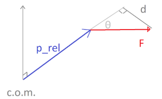
(Let’s not confuse d with the penetration depth, it only refers to the length of the triangle side indicated).
Recall that is the vector extending from the center of mass to the point of contact p, at which the force is being applied. It makes complete sense that the direction of the torque vector would be normal to the plane defined by and . It also makes sense that the magnitude of the torque (arm length) * (normal force) would be where is the angle between and .
Combining Formula 2 and Formula 3 by substitution for we obtain:

Formula 4:

Lastly, let’s assume that the force is always along the direction of the contact normal be it positive or negative, and let be the magnitude (and direction) of that force, such that:
.
If we treat and as constants over a time duration from to we can integrate Formula 4 with respect to time, to obtain:

By pulling out constants, and taking advantage of the fact that cross products are distributive, we can simplify the formula as follows:

Taking note that is a scalar value, and equal to , we can pull it out to obtain the following formula:

Formula 5: 

The quantity is what’s sometimes called “Impulsive torque” for note its similarity to the torque formula in Formula 3 (especially if you combine and to describe the impulse as a vector), and note how Formula 5 is analogous to Formula 4.

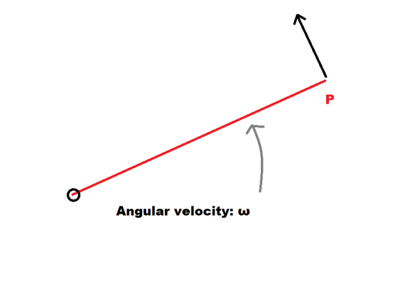
Linearizing the rotation:
We have a delta in angular velocity, but what linear velocity does that amount to at the point of contact? For this we have another geometrically intuitive result:

Formula 6:

Where is the linear velocity resulting from the rotation . Consider the following diagram to see why this makes intuitive sense:

 

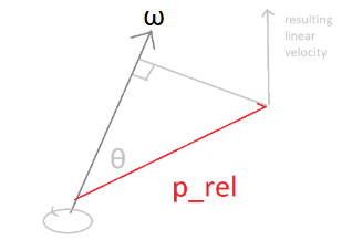
Recall that is a vector and directed along the axis of rotation, it makes complete sense that the direction would be normal to the plane defined by and . Moreover, the magnitude is given by:

Where is the angle between and .
Lastly, we need the velocity in the direction of the contact normal. So we simply take the dot product with to obtain the angular portion of the delta in closing velocity, which we call  :

Formula 7:

Note we are sometimes using quantities like: and interchangeably, and similarly for linear velocities: and . Do not confuse the with an infinitesimal or a derivative, these are just differences, subtractions, and therefore the same theory holds. With this in mind, we can replace  in Formula 7 with from Formula 5 to obtain:

Formula 8:

Note we took advantage of being a scalar, and pulled it out in front.

Putting it all together:

Combining our linear velocity as a result of rotation, together with our earlier linear result, we obtain:

Formula 9:

Note the dot product with only applies to the angular component. The impulse scalar is already assumed to be in along the direction of the contact normal.

Finally, we need to determine the delta in closing velocity between the two bodies as a result of the impulse . By our convention for closing velocity, we subtract the 2nd body (body1) velocity. However, the forces for the 2nd body are also oppositely directed and therefore the impulses are oppositely directed. Therefore, the negatives cancel and we simply add the two to obtain Formula 1:

Formula 1: 

Matrix Form

Formula 1 is a frictionless derivation that only accounts for the change in velocity along one direction. We review it because 1) it motivates the matrix derivation and 2) we will use this frictionless formula as a simplified model when resolving interpenetration.

We will use a similar derivation of Formula 1 to determine a matrix that transforms from an impulse given in contact coordinates, to a delta in velocity, also given in contact coordinates. Once we are armed with this transformation, we will see how we use it to calculate a friction-based impulse.

For this, we need to express the cross product as a matrix transformation. It turns out that for any vector , we can find a corresponding matrix such that .

Now recall Formula 5:

Note this defined the change in angular velocity as a result of an impulse in the direction scaled by the scalar . If we rename our variables to combine and into a single vector , we can write the above formula as:

Formula 5.1:

Note that was a vector in world coordinates and so in the above formula would also be in world coordinates. We want things in contact coordinates ultimately, so we’ll address this in a bit.

Once again, we must linearize the rotation to determine the change in velocity at the point of contact. So, as before we use formula 6 (again noting we can interchange and ) and substitute our result from Formula 5.1 to obtain:

Formula 5.5:

Recalling that we can reverse the order of a cross product by adding a negative sign we can rewrite this as:

Now, we can replace our cross products with with the corresponding matrix . Let’s just call it for short.  (The book refers to this as a skew matrix, since it is skew symmetric). Moreover, since we are just dealing with matrices which are associative, we can regroup the parenthesis:

Formula 6.1: 

We are almost there. Both and are in world coordinates and we want our delta velocity AND our impulse to be in contact coordinates. So if we want in contact coordinates and we have a “contact to world” matrix , we must replace in the formula above with . Moreover, we must convert the final result of the formula back to contact coordinates by left multiplying the result by . This results in the following:

Formula 7.1: 

Now comes the easy part! We have above what we call the “angular intertia”. Now we just need the “linear inertia”. Before we just scaled by so in matrix world we just need a diagonal matrix . Note this maps from contact coordinates to contact coordinates so no change of basis conversions are needed. So combining the linear and angular inertias, we obtain the total velocity delta in contact coordinates:

Formula 8.1: 

Finally, through the exact same reasoning as before, if we wish to account for the delta in closing velocity between two bodies (accounting for our closing convention of body0 velocity – body1 velocity, and the oppositely directed forces), we obtain the following sum:

Formula 9.1:

From which we have finally derived our magical inertia matrix that converts from an impulse vector in contact coordinates to a change in closing velocity vector , also in contact coordinates:

Formula 10:

Armed with this now 3 dimensional mapping, we can compute the appropriate impulse that takes friction into account, in the next section!

Computing the impulse (with friction):

Recall that our general strategy for all of the velocity resolution is to compute the impulse; the impulse that will bring about the desired delta in velocity. Now that we have a 3 dimensional version, the x component of the closing velocity (in contact coordinates), will be determined by the coefficient of restitution, and the y,z components will be determined by the friction.

The trick the book uses is as follows:
1. Compute the impulse necessary to bring about the desired change in closing velocity in the direction of the contact normal (the x axis of the contact coordinates) according to the restitution, and to completely kill the closing velocity in the and directions.
2. Check to see if there was enough friction present to stop the sliding, in which case the impulse computed by 1 is applied and we are done.
3. Otherwise, if there was not enough friction, we modify the impulse. We scale the impulse vector computed in step 1 in the yz plane only (we assume the yz direction of the modified impulse will be the same), and revise our x impulse, such that the friction equations are satisfied, and the delta in closing velocity along the contact normal (the x axis of the contact coordinates) is still what is dictated by the restitution.

Step 1:
If our initial closing velocity in contact coordinates is given by and is  our restitution, then the desired change in closing velocity is given by:

So we therefore compute the correspond impulse by solving the equation below (just take the matrix inverse):

Step 2: So how much of an impulse do we have in the direction of the yz plane of the contact coordinate system, as a result of friction? Using the coefficient of friction we have the classic formula:

Formula 11:

Where and are scalars. Once again, we can integrate the forces over a time duration to obtain an analogous formula of impulses:

Formula 12:

By Pythagoras, and by noting that in our particular case , and that  is the direction of the yz plane of the contact coordinates, we can apply the above formula to conclude the max frictional impulse:

Formula 13:

(Note we don’t need the absolute value of because we expect to be positive, as mentioned before).
Therefore, after computing in step 1, we check to see if:
is less than:
If this is so, then is an appropriate impulse and we can apply it, and we are done!
Otherwise, we compute an entirely new impulse that has the following form:

Formula 14:

Note what we have done here. We have used only to deduce the yz direction of the new impulse, and then normalized and scaled it in the yz plane according to the friction relationship. We have also introduced a new variable . We are figuring out an entirely different impulse now, and is the only variable to solve for.

Solving for it is actually quite easy. This modified impulse corresponds to a modified delta in closing velocity:

.

We actually only know the x component of , which is the delta in closing velocity based on the restitution, which let’s just call to be concise. It turns out this is all we need. We substitute for both and in the equation above, to obtain:

(Note we are using a T exponent to denote transpose as the vectors should be vertical).

If we look at the very top row of this matrix equation, we can obtain a single, scalar value equation in one variable:

Where denote the first three elements of the first row of matrix M, respectively.

Solving for we obtain:
Formula 15:

Then using Formula 14, we can use to compute the rest of the impulse, and we are done!

One final note – the approach of solving for the top row threw me the first time because I wondered “How do we know the rest of the equation is satisfied?”. The answer is “There is nothing to be satisfied”. We modify the impulse and comes out to be, whatever it comes out to be. So long as the friction equations and the top row are satisfied, we are golden.

This concludes our discussion of velocity resolution.

Resolving Interpenetration

We already discussed the details of resolving penetration in a previous  post: ““Collision Resolution 2 – resolving interpenetration” but a few newer details have come to light, and also for the sake of completeness I will review it here.

Recall that the general approach taken is to first determine the change in closing velocity
and then “fast forward time” by a time such that where is the depth of penetration.

We will need our inertia formula (not to be confused with moment of inertia) we derived before to resolve the penetration.  As briefly noted earlier, rather than use the friction-based 3×3 matrix, to work out this calculation, the book takes a simplified approach and use the frictionless Formula 1 (the friction version will be used for velocity resolution only). The formula is restated below:

Formula 1: 

Note that in this context, and for this discussion, is a scalar again (though we will see shortly, will be eliminated from our resulting formulas).

Let us refer to the entire sum in Formula 1 as :

For the purpose of this discussion we are going to need to split the above sum  into 4 pieces. Observe the left hand side of the formula  is the linear component of the sum, and the right side is the angular component. Moreover, we have two rigid bodies, each of which contributed a linear and angular component to the sum.
To concisely denote these quantities, and to mimic the implementation code for ease of comparison, we will use standard programming language array notation with indices in brackets to denote which body we are using: [0] will correspond to body0 and [1] to body1.
Let us hereby define the following variables:

These should make some intuitive sense, for these are how we derived the closing velocities in the first place, by looking at the individual linear and angular inertia of each body before we combine them into a single sum. Note, however, that the inertia quantities above map an impulse to a change in velocity in the direction of the contact normal, but not a change closing velocity anymore, since we would need to compute differences for that. This is why we need this, we want to control for individual movements as we resolve the penetration between the two bodies.

So the question now is, how much time would it take for the delta in closing velocity to cause the objects to separate by the penetration depth ? Well:

implies:

Set the right hand quantity equal to and solve for to obtain:

So how much linear motion does this result in, for each object? For this let us introduce 4 new variables, similar to our approach for inertia:

These correspond to the linear shifts in the direction of the contact normal (be it positive or negative) that will be applied for each body. The angularMove quantities, it should be noted, are 1) not the actual rotation values, but the linear motion resulting from that rotation which will be applied, 2) linear approximations of an arc, and part of why we want these quantities to be small.

Now that we have suitable notation, we note that we can multiply an inertia quantity by to find a delta in velocity. We can then multiply that delta in velocity by a time duration to find the resulting movement  (we use both of these facts a lot in the derivations below, so be clear on this):

Formula 16:

Formula 17:

The formulas for , and are analogous, but we must apply a negative sign since the forces would be oppositely directed for body1 (this is true even though we eliminated impulse from the formulas because the g in the initial t calculation would not have its sign inverted). 

Next we must determine how much rotation angularMove[0] and angularMove[1] correspond to, but there is something we must do first. Recall that the quantities are linear approximations of an arc and they are only suitable if the arc is relatively short. Sometimes, depending on the inertia tensor and mass values, the calculated angularMove could be so high it would be a bad approximation. To handle this, our algorithm will cheat a bit, and check to see if the angular move value is above some calibrated threshold, and if so, transfer some of the angularMove over to the linearMove. Yes this distorts our original reasoning a bit, but it works. We’ll cover this in the “Avoiding excessive rotation” section shortly, but for now just be aware that the angular and linear move may be modified after they are calculated, and before they are applied to the rigid bodies.

Applying the motion:

Applying the linear move quantities (after the excessive rotation modifications) is straightforward. We simply add/subtract the appropriate linear move quantity multiplied by the contact normal to body0/body1 respectively.

The rotations are a bit trickier. We can compute our delta in angular velocity from Formula 5 and multiply it by our earlier time duration . The only issue is our logic to avoid excessive rotation may have overridden the angular move values, which invalidates our time duration t (we didn’t need to recompute t for the modification to the linear move, because all we needed to know was the desired move distance, whereas we still need t to compute the change in rotation).

We therefore need to recompute based on our new angular move value. Let’s call it . This calculation is straightforward, we use an equation we saw before and solve for different variables:

Solve for to obtain:
Formula 19: .

Now we must use Formula 5 which we restate below:

Formula 5: 

We need only multiply the right hand side of Formula 5 by to obtain our resulting rotation (note the cancels out):

Formula 20:

Note that really should be denoted as and as since they each correspond to body0, but it seemed cleaner for this discussion to omit these. As before, the body1 result is analogous but we must multiply by -1 to account for the oppositely directed forces.

Lastly this rotation vector would be applied to the orientation of the respective body by using an updateByVector() function on the quaternion, or something to that effect.

We will now discuss how to avoid the excessive rotation before giving a full summary of the penetration resolution process.

Avoiding Excessive rotation:

As usual, the book uses some odd motivational reasoning that does not quite agree with the implementation (at least in my mind).

The implementation takes the following approach:
1. Set a maximum rotation threshold given in radians, let’s call it .
2. Use to compute the corresponding maximum move at the point of contact.
3. See if the originally computed angularMove value exceeds this value, and if so, transfer some of the move over to the linear move.

Only step 2. really requires comment.

Imagine for a given relative contact vector we applied a rotation of and wanted to know the corresponding linear movement at the point of contact in the direction of the contact normal .
(This happens to be very similar to the “Law of Gearing” proof).

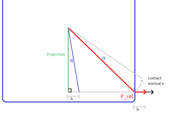
First we compute a “Projection” vector, by subtracting from the component in the direction of .

If we visualize the resulting right triangle, formed by and the Projection vector, as a rigid body, we can see that the base of the 90 degree corner would have (approximately, for small rotations) the same shift as the shift at the point of contact in the direction of the contact normal.

The shift and maximum allowable angular move would therefore be:

Finally, since is usually calibrated as a small angle, we can approximate with (also is constant, so it especially doesn’t matter). We therefore obtain the following formula found in the code implementation:

Formula 21: .

Now let’s concisely summarize our algorithm and the appropriate formulas used.

Summary of penetration resolution:

 Step 1: Compute the linearMove and angularMove values according to Formulas 16 & 17 (and the analogous formulas for body1), utilizing only the inertia quantities.

Step 2: Use formula 21 to see if the angularMove values are too high, and transfer the excess over to linearMove.

Step 3: Apply the linearMove shifts directly to the positions of the rigid bodies.

Step 4: compute the applied rotations using Formula 20 (and the analogous result for body1), utilizing only the angularMove and angularInertia quantities.

Independence of velocity & penetration resolution:

Note that our formulas for penetration resolution ended up not depending on the impulse value . This is serendipitous, because it means we can resolve a collision independent of the velocity situation. There are some occasions, when a collision could occur, but the closing velocity may be positive. Under such a circumstance, we would not want to perform a velocity resolution, but we MAY want to resolve the penetration, and by the above observation, we may do so.

CODE REVIEW:

The following code is cited  from Ian Millington’s Github. I do not own this code:

https://github.com/idmillington/cyclone-physics/blob/master/src/contacts.cpp#L437

All of the calculations should follow fairly closely the formulas that were presented. Keep in mind the corrections that were noted before, such as the contact normal not being oriented from body0 to body1 as the book stated.

Fortunately Ian Millington used your preferred matrix convention:
1. The matrix multiplication by a vector uses right multiplied by a vertical vector – producing a linear combination of the matrix columns.
2. The  *= operator is overloaded to mean “right multiply by” so A *= B == A*B
3. The elements of the matrix are represented as a 1d array of length n*n and proceed in row order. i.e. M[0],M[1],M[2] correspond to the first

Resolving velocity:

 

Comments:

1. On line 311 it says “Build the matrix to convert contact impulse to change in velocity in world coordinates” this threw me a bit. I thought “contact impulse” meant an impulse vector in contact coordinates, but I think it means to say “impulse as a result of the contact”. The associated matrix is a world-to-world mapping, and agrees with our derivations.
2. In the formula for impulseContact.x on line 369, desiredDeltaVelocity corresponds to in Formula 15.

Resolving interpenetration:

 

Robust Stencil Shadow Volumes

Shown above: My CPU (Soon to be GPU) implementation of the algorithm discussed below. Note the little white sphere is not actually casting light, it is merely to illustrate shadow calculation.

Hello friends!

Progress is slowed due to me recently receiving full-time employment as a software developer here in Philadelphia. But the show must go on!

In this update I am going to talk about Stencil Shadow Volumes. More specifically:

1. The traditional stencil shadow volume technique
2. The necessary constraints for the technique
3. A modified algorithm
4. Implementation issues for both algorithms
5. My implementation of the modified algorithm
6. Possible improvements for my implementation

1. Traditional Stencil Shadow Volumes.
Lets recall the basics of the stencil shadow volumes technique. There are two components to the process: projecting a closed solid volume representing the shadowed region created by an occluder (See OGLDev Tutorial 39), and using this volume to update the stencil buffer and determine which pixels are shadowed (See OGLDev Tutorial 40). The later part is straightforward and is based on a “depth-fail” test. The first part is trickier and depends on the mesh topology.

Projecting a shadow-volume is performed by determining the ‘silhouette’ or outline of an object from the light’s point of view. The silhouette is composed of a series of ‘silhouette edges’, defined as edges that connect a light-facing (hereafter referred to as a ‘front-facing’) triangle to a non-light-facing (back-facing) triangle. Each silhouette-edge is extruded/projected behind the object (from the light’s point of view) to form a quad primitive, and these quads form the sides of the shadow volume. The developer decides whether to designate front or back faces of the original mesh to form the front and back ‘caps’ of the volume (back faces work better if the light source moves inside the mesh, but cost the extra rendering time). The back cap is computed by projecting the front cap and reversing the winding. The details can be found in the OGLDEV tutorial.

So there we have it. Given a light source, we can calculate a closed shadow volume that can be used with the stencil buffer to mark shadowed pixels. There are, however, a few subtle assumptions which impose constraints.

2. The Constaints:
One key requirement is that shadow volumes most form one (or several) closed volumes. For this it is necessary that the mesh be a closed surface, or a “two-manifold” as most of the literature describes it (exact constraints vary per implementation).

Another more subtle constraint exists in the winding of the mesh. The winding of a face/triangle is the order in which its vertices are rendered. Note this does not directly determine whether a face is front or back-facing which was a key source of confusion for me in the past. Reversing the winding of a face will flip it from front-to-back facing, or vice-verse, but it depends on the position of the vertices and the viewpoint. The winding of a face determines the ‘direction’ of its edges (with respect to that face), and in the case of silhouette edges, determines the winding of the projected quad, that forms a side of the shadow-volume.

For example, suppose (v0,v2,v4) is a front-facing triangle, and (v0,v2) is a silhouette edge. Then (v0,v2,v4) forms a front-cap of the volume, (P(v2),P(v0),P(v4)) forms a back-cap (where P denotes the projection of the vertex from the lights point of view), and (v2,v0,P(v0),P(v2)) forms a quad; one of the sides of the shadow-volume. Note how the winding of the projected quad is opposite that of the adjacent front and back caps. For proper stencil buffer based shadow calculation, the shadow volume must obey the property that adjacent faces have opposite winding. For this reason (and others) it is necessary that all adjacent faces on the original mesh have opposite winding.

Not surprisingly, the model’s I purchased do not satisfy these constraints. So I set out to find a more robust algorithm.

3. A Modified Algorithm:
This paper: http://hungryspoon.com/PX_web/paper/paper.pdf was recommended to me by RAZORUNREAL from GameDev.net, and seems to place literally no constraints on the mesh. I will motivate this algorithm despite a conspicuous lack of motivation by its author.

Suppose we used a brute force approach to render shadow volumes. Rather than rendering a single volume around the silhouette from the light’s point-of-view, one could simply label every edge of every front facing-triangle as a silhouette edge, effectively projecting a single (triangular) shadow volume for every (front-facing) triangle. This would work, as each volume would certainly be closed (and multiple closed volumes are allowed). This is obviously expensive and there are even more edges than faces in a mesh. However! One might observe that two front-facing, oppositely-wound triangles that share an edge e, would both project an identical, but oppositely wound quad from e. Since these quads ultimately increment or decrement the stencil buffer based on their winding, the net effect of these two quads is zero. So oppositely wound quads ‘cancel out’ each other. For this reason, if we determine the net number of projected-quads along each edge (after cancellations) prior to rendering them, we can save significant execution time. Moreover, we always obtain perfect, closed volumes, with no constraints on winding, or the maximum number of adjacent faces.

The precise algorithm presented in the paper is outlined below. Note, consistent with what I’ve written above, we designate front-facing triangles as the caps of the shadow volumes. Keep in mind this means only light-facing triangles cast shadows.

Once after loading mesh:
Label each edge with an arbitrary direction-label, and initialize a signed counter variable for that edge to 0.

before each rendering: 

for each face f in mesh:
{
   if f is back-facing, skip it.
   
   else for each edge e in f :
   {
     if the direction-label of e agrees with the winding of f:
	increment e.counter
     else
        decrement e.counter
   }

}

generating shadow volume:

for each edge in mesh:
  while (edge counter > 0)
    render silhouette edge with same* winding as edge direction-label
    decrement edge counter
  while (edge counter < 0)
    render silhouette edge with opposite* winding as edge direction-label 

Note, depending on how you wind the front-facing caps, you may want to exchange the positions of ‘same’ and ‘opposite’ in the above description. I think the paper got these backwards. Just remember that adjacent faces in the shadow volume must have opposite winding and make sure this is achieved.

This algorithm has some surprising features. In particular:

1. There is no need to keep track of or process ‘adjacent’ faces.
2. Winding is constant regardless of whether a face is front or back-facing. Thus a given face’s contribution to its edge counters is determined even before it is rendered. It is merely a question of if the face is front-facing that determines whether or not the contributions are made.
3. The same silhouette edge is sometimes rendered repeatedly. This implies the existence of multiple closed volumes.

The author of this paper asserts that there are no-known constraints on the mesh topology (which we effectively proved in motivation), and renders a minimal number of silhouette edges. so this is essentially a perfect algorithm. A perfect implementation, however, is a separate story.

4. Implementation Issues:
Traditional Algorithm implementation:
Currently, OpenGL provides a special, per-primitive shader called the ‘geometry shader’ which can be used to quickly determine and generate silhouette edges in the traditional algorithm. The geometry shader is handed 3 vertices for the triangle, plus 3 more, to determine the adjacent triangles. See figure 1 below.

The geometry shader can be programmed to emit a silhouette edge for a given, front-facing triangle, if the adjacent triangle is back facing. The front faces of the mesh are used to compute and render the front and back caps of the shadow volume, and the shader automatically detects and generates the silhouette edges on those faces. This way, the silhouette edges are computed in parallel by the GPU. OpenGL literally has dedicated features for the traditional silhouette detection algorithm (i.e. GL_TRIANGLE_ADJACENCIES) so a very fast implementation is possible.

5. Modified algorithm implementation:The main problem with the modified algorithm described above is that it does not fit neatly into the OpenGL pipeline. How do you keep a counter for each edge and update it using the GPU?

My solution is to proceed as in the traditional algorithm and have the geometry shader auto-generate quads. At each front-face, deduce the value of the counter for its edges by considering the adjacent triangles. To deduce the counter values, however, I need to know the winding of the adjacent faces and here we have a problem.

Consider Figure 1 again. While the triangle (0,2,4) has explicit winding (because they are supplied in order to the geometry shader), there is no way of knowing the winding of the adjacent triangles. For example, is the winding of triangle {0,1,2} given by (0,1,2) or (0,2,1)? In fact, to deduce that an adjacent face is back facing in the traditional algorithm, you need to assume it has opposite winding to the given face!

Turns out this is a hint in disguise. Recall from figure 1 that a triangle (v0,v2,v4) is supplied to the geometry shader with the vertices of its adjacent triangles (V1,v3,v5). If an edge, say (v0,v2) has no adjacent triangle, you can choose to represent this by letting v1 = v4. The geometry shader can check for this to see if an edge ‘has an adjacent triangle’ or not.

With this flexibility, we can mandate that we only supply an adjacent triangle to the geometry shader if the adjacent triangle is oppositely wound to the given face (v0,v2,v4). So when considering the edge (v0,v2), the GS would first check if v1 != v4 and if so, would assume (v0,v1,v2) is an oppositely wound, adjacent triangle. Conversely if (v1 = v4), it will be assumed that edge (v0,v2) is connected to (one or more) identically wound triangles. For the sake of discussion, in the context of the geometry shader, stating that a triangle ‘has no adjacent triangle’ along an edge e, will simply mean an adjacent triangle was not supplied, not necessarily that it doesn’t exist. Keep in mind, all of this adjacency information is pre-computed based on winding, and stored in the index buffer.

This resolves the ambiguity of winding and we can therefore determine how each face will contribute to the edge counters on a face-to-face basis. Rather than keeping a counter variable, we just emit quads with appropriate winding. In some cases, redundant quads will be rendered and ‘canceled out’ but this will be very infrequent.

5. My implementation:
We now have enough machinery to describe my algorithm. For now let’s assume the mesh has a maximum of 2 triangles adjacent to each edge.

Once after loading the mesh:
Configure the index buffer so that adjacent triangles are provided only for oppositely wound triangles.

During rendering:
(geometry shader):
for each face f:
  if f is back facing, skip it and continue to next face
  else for each edge e in f:
	if (f has an adjacent AND back-facing triangle along e) OR (f has no adjacent triangle along e):
		project a quad from e, with same winding as f
  
	

The idea is this. According to the modified algorithm, if two adjacent triangles along an edge e are oppositely wound, then e will have its counter modified if and only if one is front-facing and the other is back-facing. The counter will indicate to project a quad from e with the same winding as the (front-facing) triangle. This geometry shader achieves exactly that. Note it will only process the front-facing triangles.

On the other hand, suppose there are one or several identically wound triangles adjacent to an edge e. The number of times the edge counter is incremented (or decremented) corresponds to the number of these triangles that are front facing ‘N’. The counter will indicate to project N quads from e with the same winding as the triangles. Therefore in our geometry shader any edge connected to identically wound triangles (which the geometry shader will detect by having ‘no adjacencies’) should project an identically wound quad, once for each front-facing triangle adjacent to it.

In short, this is almost exactly the same as the brute force algorithm. We just pair off oppositely wound, adjacent triangles to take care of the canceling effect where it most frequently occurs. Turns out that if there are no more than two triangles adjacent to a given edge, this will behave exactly as the modified algorithm! 🙂

6. Possible improvementsIf there are potentially more than two adjacent triangles along an edge, the algorithm could still work. The modifications would be:

For a given edge, pair off as many oppositely wound triangles as possible by marking them as adjacent. Any remaining, unpaired triangles are marked with ‘no adjacencies’. Note in this case, a triangle may be adjacent to an oppositely wound triangle, but marked with ‘no adjacencies’, because the adjacent triangle was paired off with another, oppositely wound triangle along the same edge. This is where my implementation may not behave optimally, but the net number of rendered quads will still be correct. Moreover, this occurrence of more than two faces adjacent to an edge should be very infrequent and not pose any performance issues.

Lastly its worth mentioning that stipulating only light-facing triangles cast shadows can look odd because triangles invisible to the viewer may cast shadows (if culling is enabled) or visible triangles may not cast shadows (culling disabled). To address this, another possible improvement is just to iterate the algorithm twice. Once for front-facing triangles, and the other for back-facing. The algorithm would need to invert the windings, and reverse the roles of ‘front’ and ‘back’ facing accordingly. This would obviously be a more expensive operation but the technique could be optional as the need is infrequent.

The video above shows a preliminary CPU implementation of my algorithm, used to cast a shadow. My GPU implementation is being developed to fit inside my deferred renderer which I am currently working on.

That’s all, folks!

Update: A series of unfortunate discoveries

Hello, friends!

Its been a while since I posted an update and much has changed with the project. I had a series of unfortunate discoveries that forced me to re-think a lot of my design choices and ultimately led to a lot of studying. Here were some of the unfortunate discoveries and how I’ve dealt with them:

1. My artist doesn’t produce any work.
Moreover he went and had a baby and has no time anymore! As a result I was forced to obtain models from TurboSquid.com. While it has some decent (mostly non-animated) models for cheap, all of the models I purchased had at least one bizarre issue, which leads me to my second unfortunate discovery:

2. ASSIMP is glitchy and unpredictable with models created in Maya or 3DS Max
I was extremely sad to admit this because I am a huge fan of the Open Asset Import Library. I blame Autodesk! Since most of the pre-made models I find are available in Autodesk proprietary formats which break after file type conversion, I decided to switch to the Autodesk FBX SDK for loading models. Since the FBX file format and the SDK is owned and maintained by Autodesk, this guarantees compatibility with any models created in Maya or 3DS Max. So I took some time out to learn the FBX SDK, which brings me to my 3rd unfortunate discovery:

Or, in case the image didn’t load:
3. The FBX SDK is hideously complicated and has very few available learning resources.
It appears that Autodesk has a nasty habit of revamping the SDK too frequently and so basically no one knows how it works. Even members of the FBX team on the message boards are often unable to elaborate on the subtleties of the SDK. Sadly I could see no alternative so I spent over a full month immersing myself in the available example code and running experiments to unravel the details. Skeletal animation was one of the most complicated issues to understand as FBX uses a much more sophisticated deformation system than ASSIMP. After a lot of frustration, I eventually produced this video to reinforce, save, and share the knowledge.

Not surprisingly, there is one extra detail I missed pertaining to skinning in fbx as it is just ridiculously complex. Autodesk features FBX in almost all of their products and I doubt any one person understands every nuance of the sdk. It took a lot of work but at this point it seemed that I had a strong enough understanding for what I needed to do. Shortly after I escaped the perilous dungeons of this sdk I made another frightening discussion:

4. I no longer know OpenGL!!!

I learned OpenGL from the RedBook and other sources where Immediate Mode was still popular. That is, before Vertex Buffers and GPU Shaders were the norm. I didn’t really intend to make the graphics at all sophisticated for this project, but the number of vertex deformations required by these models is just too high to be done in the CPU. It is a topic I was long intimidated by but I decided to bite the bullet and learn all I could about shaders. This brings us to number 5.

5. OpenGL Shaders are too awesome to ignore!
I went through every single tutorial on this site: http://ogldev.atspace.co.uk/ which I’d highly recommend to anyone.
After learning so much about shaders, it was clear to me I had to implement at least a few of the effects that make the visuals in modern games really pop. Specifically I’m hoping to implement:

1. Deferred Shading
2. Normal Mapping
3. Shadow Maps for Spot Light shadows
4. Cascaded Shadow Maps for global direction (sun) light shadows
5. Stencil Shadow Volumes for point light shadows
6. Basic gpu tessellation with displacement mapping (optional)

Here is a short clip of when I first got shadow maps to work, together with skelatel animation, using the FBX SDK:

the shadow occasionally disappears near the feet but I have since resolved that issue.

Lastly, the final unfortunate discovery was:

6. An impulse based physics engine is bad for rag-doll physics

Although I loved every moment of learning the Cyclone Physics engine and learning how it was built from the ground up from my textbook, an LCP constraint solver is clearly much more stable and suitable for this application. Therefore I have examined two physics LCP based physics engines: ODE and Bullet. ODE is fantastic and has everything I need but seems to be just a little bit glitchy, unpredictable and fading into obscurity, so it seems Bullet will be the engine of choice for this project.

Well that about brings us up to date! I hope to soon follow up with an update about my graphics engine. Goodnight all!

Collision Detection – Capsules

Very excited to doing some coding again! Still have a little reading left to cover in my textbook, but the physics engine is complete so I can start playing with it.

The first thing I want to do is enable collision detection between human characters.

As I may have mentioned, we often approximate the collision boundary for complicated objects using simpler shapes we call ‘primitives’ like spheres, boxes, convex polyhedra, and sometimes combinations of these.

So I was thinking about what kind of primitive would be best for a human character. I thought about using a bounding box, but the sharp corners would probably get caught on objects in the scene.

Then I had a better idea. A rounded “capsule” shape

It approximates the shape of the body fairly well, its smooth shape keeps it from getting snagged on sharp objects, and collision checking is fairly straightforward. So its win,win,win. I also talked to guys at gamedev.net about it, and they said this is actually a pretty standard approach. So I went ahead with it!

In my implementation, my capsule is technically a composition of a cyllinder and two cyclone collision spheres.

Sphere/halfspace collisions simply check for collisions with the end spheres. i.e. the spheres will hit the floor before the mid section does.

Capsule/Capsule Collisions are slightly more involved. These capsules have the nice property that they are the set of all points a distance r from the line segment which forms the axis of the cyllinder. This means we only need to find the points on the two line segments that are closets, and check if their distance apart is greater or less than the sum of their radii. This forms a 2 dimensional boundary value problem, which equates to finding the point of nearest approach of two infinite lines (zero derivitive) and 4 point-on-line-nearest-to-point checks (boundaries) and then taking the minimum. Not that complicated.

Here’s a short video clip of me testing capsule collisions :]

Two final comments:

I use the inertia tensor for a cyllinder (with no spherical caps) for this shape, which is described in the appendix of my textbook.

Second, for capsules with very small radii, the very small mass/intertia tensor, plus frictional impulses, can result in the capsule spinning very rapidly along its axis, to the point where it litterally behaves like a top. Limiting the smallness of the intertia tensor (even if the size of the object is smaller) seems to work. Perhaps I could add additional angular velocity damping, exclusively for velocity in the direction of the axis.

Hello! So the bad news is school has started up again, and that means less time for game-dev study. But the good news is I am at the tail-end of my physics programming textbook, so I may actually be coding some stuff soon! :]

The last chapter with any real substance in the textbook is Friction and Resting Contacts. (Objects that are sitting on, sliding over eachother). Next chapter contains some minor tweaks for optimization and stability. Then a few chapters on other topics like 2d physics, that don’t pertain directly to the Cyclone physics engine.

The chapter on friction has been pretty comprehensive! But there are one or two points which I thought were worthy of comment.
The first topic has to do with Stability. A crucial part of our collision resolution is velocity resolution. And a key technique we used was to calculate the desired change in velocity between two colliding objects, at their contact point. This depended on the coefficient of restitution.

Velocity depends on pre-existing velocity, plus additional velocity due to acceleration in the last frame. It is often useful to remove the portion due to acceleration. Why? Because objects that are touching and/or at rest, will want to accelerate into eachother due to gravity or other potential forces. So it makes more sense to ignore this component. If no contacts are present, the acceleration will contribute to the velocity over a period of time, so there is no real harm in doing this.

Effectively, we treat the initial closing velocity as if the velocity due to acceleration, were not there (by subtracting it)
That is:

Where is the desired separating velocity after the collision, and is the coefficient of restitution.

But we want the change in velocity from what the closing velocity initially is () to the final separating velocity after the collision () Subtracting thus gives:

The book uses this formula in the implementation but not in the motivation (not sure why)
Note I’m somewhat abusing the language ‘separating’ and ‘closing’ velocity. They are supposed to be negatives of eachother. I am really taking them to mean the separating velocity. I just like to use this to distinguish between velocities before and after the collision, as objects are initially closing and then separating after collision.

Now we need to remember that these are the velocities in the direction of the contact normal. That is, the x-componant of the closing velocity in contact coordinates.

This brings us to our next topic. When discussing velocity resolution, we found a formula for the amount of velocity resulting from a unit of impulse (impulse in the direction of the contact normal). We then inverted the result to find the ammount of impulse required in this direction to bring about the desired change in velocity.

While we were only interested in the quantities in the direction of the contact normal, nothing about the formulas we used were dependent on using that specific direction. We could have found the change in velocity due to a unit impulse, with impulse in the direction of the y or z axis in contact coordinates.

So, suppose we have an impulse applied at the contact point of an object:

And we want to know the resulting change in velocity:
.
We can use the same formulas (replacing the contact normal with the appropriate vector) to compute the amount of impulse needed. The convenient part is that the 3 calculations which perform this transformation can be described as a matrix which does all three at once. This is done by converting cross products into equivalent matrix transformations, the appropriate change-of-basis matrices, and so on. The details are in the textbook and not very complicated. The point is we end up with a matrix such that:

Which we can invert to obtain:

So we can figure out how much impulse to apply given our desired change in velocity. Remember the x component of this velocity is in contact coordinates, and so the y,z components are the changes in the ‘sliding’ velocity along the surface (which will depend on friction)

We computed the desired change in velocity for the x-component earlier (using the coefficient of restitution). So here is the approch the book uses:
1. Let the desired change in velocity for x be what we already computed (based on coefficient of restitution).
2. Let the desired change in velocity for y,z be exactly enough to stop the object from sliding, as if the friction stopped it entirely (y,z components of velocity of contact point, in contact coordinates)
3. Determine if (2) was valid, by checking if there was enough frictional impulse (frictional force, integrated over time) to stop the object.
4. If 2 was not valid, we recalculate the impulse due to dynamic friction.

Here’s how we determine if there was enough force to stop an object. The maximum static friction in the contact plane will be given by:

Note the x direction of force gives the force against the surface, which contributes to friction. Integrating both sides with respect to time gives:

Because impulse is just the integral of force over time. This gives us a neat relationship between impulses.
Thus after step 2, if:

Then static friction is no longer sufficient to stop the object. So we have applied too much impulse.

For this, we use dynamic friction. In this case, we make an assumption. The assumption is that the direction of the resisting forces due to friction as the object slides (equivalently, the frictional impulse) is in the same direction as the frictional impulse required to stop the object entirely. I can’t find a rigorous proof of this, but I think its intuitive enough to accept.

The impulse due to dynamic friction obeys the same relationship, just with a potentially different value of . So the relationship between the impulse in the x direction, and other two impulses should be:

The only difference now, is that before the ‘static’ frictional impulse was limited to this, and stopped the object entirely if planer impulse was insufficient. In this case, the frictional impulse is EXACTLY this. So we have to modify the impulse accordingly.

Together with the last assumption, we can easily find the y and z impulses that satisfy this:

This will change the delta velocity in the y,z direction, which is good! Because these are unknown. Before, we had 3 known changes in velocity and wanted to determine 3 unknown impules. Now we have two known impulses, (sort of) and one known change in velocity (in the x-direction) and we want to determine the others. I said sort of because the other two impulses depend on our x impulse, which we are about to determine.

Returning to our earlier equation, we know:

applying our modifications we have:

(T means transpose)
Left multiplying by gives us:

If we look at the very top row of this product, we are left with an equation where the only unknown is . Solving for its value, you can obtain the formula used in the implementation, and shown in the textbook. We now know all the impulses we need to apply. It is not necessary to calculate the other two components of velocity, as finding the impulse was our only objective.

This completes the discussion of friction. Most of the chapter was pretty comprehensive but the very last bit about how to determine was left out entirely.

The very last thing I think is worthy of mention is related to what I mentioned earlier, and is in the next chapter on Stability. We omitted velocity due to acceleration when calculating the desired change in velocity. When calculating the separating velocity prior to this, the book decides to remove the velocity due to acceleration in the direction of the contact normal and keep only the planer component. To me, this seems to negate the need for the aforementioned step, and I feel as if too much velocity is removed, but I’ll need to think about this more carefully before I can comment on it. But it shouldn’t affect things too dramatically even if its not 100% precise.

Speaking of not being precise, there is one typo in “contacts.cpp” in the calculateDesiredDeltaVelocity function in the source code (but not in the text)

    if (body[0]->getAwake())
    {
        // 'velocityFromAcc=' was missing.
        velocityFromAcc= body[0]->getLastFrameAcceleration() * duration * contactNormal;
    }

See page 393 of the textbook to see this is correct.

Well thats all for now. This will most likely be my last major update on this textbook. Then we can move on to some more exciting stuff! :]

Collision Resolution 2 – resolving interpenetration

There are various approaches for how to move the objects apart so they no longer interpenetrate, which are discussed in my textbook. The approach used in the book is to try to determine how the new velocity of each object, as a result of the collision, will cause them to separate. The resulting motion is then “fastforwarded” until they separate. That is, we determine the ammount of time it would take the objects to separate, and then instantaneously apply the motion that would occur during this time. The notion of ‘time’ is not mentioned in the textbook. In fact not many details were given at all. But this notion of skipping forward in time agrees with the books impelmentation 100%. The book calls this method “non-linear projection”

When you consider that two objects that are collding with a given relative velocity, can be going at any speed in world velocity, this can all get a little confusing. So to keep things easy to visualize, consider two stationary objects that are suddenly pushed apart by some impulse . Then their change in separating velocity IS their separating velocity.

In my last update, we discovered a relationship between the change in separating velocity and the impulse.

The sum is messy and large so I’ll call it as the book does.

The contact data includes a penetration depth which gives the ammount of motion in the direction of the contact normal, needed to separate the objects.

So consider the ammount of time needed for the objects to separate:

Which gives:

From our last update, we determined that for each object, as a result of the impulse the changes in linear velocity at the contact point, as a result of linear and angular velocty are:

and

respectively. The book calls these quantities the linear and angular inertia when so with this notation we have:

and

The resulting motion after seconds is therefore:

and

Note how the impulse cancels out! This means the relative rates of how the objects separate is independent of the intensity of the impulse.

For the second quantity, it is important to realize this is the linear motion at the contact point as a result of rotation (by a small ammount so curvative doesn’t come into play. More on this later). Thus, while the linear move can be applied directly to the body’s position directly, the angular move needs to be converted into a rotation.

The book, however, uses to deduce an alternate formula for .
By definition:
and so:

which gives:

Moreover, we know from our last update that:

thus the total change in motion over time t is given by:

We can now update the objects orientation quaternion using the ‘updateByVector’ function. This will rotate the orientation by .

One question I had was why not use the original formula: instead of recomputing based on the angular move? I believe the reason is due to what is discussed in the next section (14.3.3) “Avoiding Over Rotation”

So far, we have been using the instantaneous velocity of the contact point on a given rigid body, to linearly approximate where it will be a short time interval afterward. That is, we are using a line to approximate what is actually a circular arc. As the line gets longer, the disagreement between the line and the arc gets worse.

The solution the book uses is to set a limit on how big the angular move (the linear motion that results from rotation) can be. If it is too large, the excess is transferred over to linear motion instead so the total move is not changed. This is farily well explained so see the book for details. But the fact that the linear and angular move undergo some recalculation, I think, is the only reason we recalcualted based on the angular move value.

So we now know how to resolve collisions for a given contact. The next topic will be how to resolve the entire list of contacts using this procedure for each individual pair. I’ll most likely write about it, depending on how well explained it is.

Collision Resolution 1 – resolving velocity

Okay! This is probably going to be a pretty critical update! The topics here are from the first half of chapter 14 in my textbook. As is usually the case for my book related updates, I’m fleshing out the details the book chose to omit. This took a little time to unravel so I want to record my details here.

This post should require a lot of math, and so I’m going to stop being lazy and start using this site’s latex capabilities.

So, what is “collision resolution anyway”. Well the collision detection system is supposed to give us a list of contacts between interpenetrating objects. Each “contact” is a data structure consisting of:
(1) the two rigid bodies that are colliding
(2) a contact point : a somewhat rough idea of where the objects touch
(3) a contact normal : a vector that gives the direction of the forces that the objects are exerting on eachother as they collide (this also is can be somewhat roughly estimated by the collision detection system)
(4) penetration depth
(5) other relavent data such as coefficient of restitution and friction.
Note the book’s choice of variable names will not always agree with mine.

The “collision resolution” process uses this data to first, determine how the velocity of each body changes as a result of the collision (both rotational and linear) and update them accordingly. The second part is to move the obects apart by the penetration depth.

The first topic is “impulse”. So we know from newtons law that:

and if we integrate both sides with respect to time, we obtain:

Now, the right hand side is what is typically called the “linear impulse” which is actually the change in linear momentum from time to . In the context of a collision, this means the force the objects exert on eachother as they collide (and compress slightly) between times to , given by , result in a change in linear momentum, given by the integral of this force over that time interval.

In addition to linear impulse, an angular impulse or “impulsive torque” will also occur; a twisting force that changes the rotation speed of each body. These two together make the collision resolution fairly complex but there is a simplification that can be made. If we assume the forces exerted between the two objects as they collide are always in the direction of the contact normal, then we can think of the integral of force over time as a scaler quantity. Moreover, allthough the linear impulse and impulse torque will be different, this sum (or integral) of forces accumulated during the instant of collision, is responsible for both.

The book uses for the linear impulse, but I will instead let and treat it as a scaler quantity. This (similar to the book’s language) is what I will call the impulse. I will add the prefix “linear” or “angular” otherwise.

For “impulsive torque” we know from the rotational form of Newtons second law that:

where is the moment of intertia tensor. Moreover, we have a formula to compute torque:

Combining these and solving for gives:

and now, by assuming to be constant (and by the fact that cross products are distributive), we integrate both sides with respect to time to obtain:

(Note we have a definite integral and so the result is and not )
The integral on the left side is the impulse! But in vector form. So we can write this as:

Where is the impulse scaler, and is the contact normal.

So lets look at our resulting equations:

and

Note I pulled the scaler out in front.
The important result here is that the resulting change in angular and linear velocity can be computed before the impulse is known and then scaled by . So the book first computes these changes per unit of impulse (by letting ) and then scaling the result once the impulse is known.

So the next question is, how is determined?

Calculating the impulse g
We deduce the impulse as follows: From the coefficient of restitution, we can deduce a desired change in separating velocty at the contact point. That is the linear separating velocity in the direction of the contact normal. Using the results above (and a little extra work) we can deduce how much impulse is needed to bring about this change.

Desired change in separating velocity:
The coefficient of restitution gives a relationship between separating velocity before and after a collision:
subtracting from both sides gives:

We can determine by calculating the initial closing velocity; the closing velocity of the two points on the rigid bodies at the point of contact, in the direction of the contact normal. This isn’t hard to compute and its explained on page 352 of the textbook, but I believe there is a typo. They compute the velocity at the contact point on the first rigid body and give a simple, intuitive formula. But they say to do the same for the second body and add the two. It seems clear to me that you must subtract the two. Otherwise, two objects approaching eachoter with velocity 1 and -1 respectively would have a closing velocity of 0. Makes no sense.

We are now halfway to deducing the impulse. We know our desired in the direction of the contact normal, and now we just need to know how much impulse will make this happen. We can compute this almost immediately from our earlier result. First lets determine the change in velocity for a particular body in the direction of the contact normal.
We have:
this is already in the direction of the contact normal and so this contribues:

to the change in velocity. The rotational component is a bit more involved, we have above a formula for but to get the resulting change in linear velocity at the contact point, we must first cross it with the relative position vector. Then we dot it with the contact normal to get the component in that direction:

So we just add the two to get the desired velocity. For the second body, we do the same only we must invert the sign of the impulse vector. However, since we subtract the two velocities to get the relative velocity, the sign changes cancel out. Thus we have:

where the sum is taken over each rigid body. We can now easily solve for and we are done!

Okay. I’ll discuss resolving interpenetration in my next update, but first two quick comments about some things I left out.

In this chapter the book introduces a “contact coordinate system” which is a coordinate system located at the point of contact, who’s x-axis is in the direction of the contact normal. This isn’t really used much in this section, but will be important later for friction. The only difference this will make will be that rather than dotting a vector with the contact normal, we’ll get the x-component of the vector in contact coordinate system, after transforming it by a world-to-contact-coordinates matrix.

Second, in most of the theory and code, the textbook speaks of the change in velocity ‘per unit of impulse’. So most of the formulas I explained look the same except the g is absent since they let .

In closing here’s a summary of how all these steps come together:
(1) calculate closing velocity at contact point
(2) deduce desired change in velocity from (1) and coefficient of restitution
(3) calculate how much impulse must be applied to bring about this change
(4) from this impulse, calculate change in linear and anguar velocity

Narrow Phase collision detection(2) Separating Axis Test implementation

So my textbook merely implements the SAT algorithm for two boxes, and since I intend to implement the algorithm for general polyhedra, I want to understand it very well. The textbook also simplifies the code in their description, instead of explaining the code in the actual implementation. So its on me to figure out everything thats happening.

So I intend to step through the code piece by piece until all of it is clear.

Before I begin, I wanted to point out an apparent disagreement between the textbook and the code, regarding normal directions. Whenever a collision occurs, the details of the collision are saved in a contact data structure which saves the pairs of bodies in the collision, the collision normal vector, and other details. The book states (p298) that by convention, the collision normal will point from object one to object two. However, the code consistently seems to do the opposite, and direct it from two to one.

For example, observe the full code for the Sphere-Sphere collision detectin algorithm:

unsigned CollisionDetector::sphereAndSphere(
    const CollisionSphere &one,
    const CollisionSphere &two,
    CollisionData *data
    )
{
    // Make sure we have contacts
    if (data->contactsLeft <= 0) return 0;

    // Cache the sphere positions
    Vector3 positionOne = one.getAxis(3);
    Vector3 positionTwo = two.getAxis(3);

    // Find the vector between the objects
    Vector3 midline = positionOne - positionTwo;
    real size = midline.magnitude();

    // See if it is large enough.
    if (size <= 0.0f || size >= one.radius+two.radius)
    {
        return 0;
    }

    // We manually create the normal, because we have the
    // size to hand.
    Vector3 normal = midline * (((real)1.0)/size);

    Contact* contact = data->contacts;
    contact->contactNormal = normal;
    contact->contactPoint = positionOne + midline * (real)0.5;
    contact->penetration = (one.radius+two.radius - size);
    contact->setBodyData(one.body, two.body,
        data->friction, data->restitution);

    data->addContacts(1);
    return 1;
}

midLine clearly points from sphere one to sphere two and it is used as the contact normal, even though one and two are registered in that order, as the pair of objects in the collision. Moreover, the normal appears to be directed from two to one everywhere in the code, despite the book explicitly stating otherwise. So I suspect this was an error.

I will therefore assume that the correct orientation of the normal points from object two to object one.

The first function in the implementation is to project a box onto a given axis:

static inline real transformToAxis(
    const CollisionBox &box,
    const Vector3 &axis
    )
{
    return
        box.halfSize.x * real_abs(axis * box.getAxis(0)) +
        box.halfSize.y * real_abs(axis * box.getAxis(1)) +
        box.halfSize.z * real_abs(axis * box.getAxis(2));
}

Note halfSize is just a vector giving the half-length of the box in the direction of the corresponding axis in its local coordinate system.
To understand the geometry, note this is equivalent to:

	return 0.5*
	(
        real_abs(axis * (2*box.halfSize.x * box.getAxis(0))) +
        real_abs(axis * (2*box.halfSize.y * box.getAxis(1))) +
        real_abs(axis * (2*box.halfSize.z * box.getAxis(2)))
	);

See the image below for an illustration of the reasoning behind this.

In other words, each of the three sides of the box is projected onto the axis and added together. The three will each compensate for portions of the projection
that were missed in the other two directions. We are really only interested in the total length. Half the total length, in fact.
And so the first code snippet gives the result we want.

I doubt such an elegant function can be used for general polyhedra, however. So an equivalent function would probably be sligthly more involved.

The next function in the implementation performs a SAT(seprating axis test) for two boxes on a given axis:

static inline bool overlapOnAxis(
    const CollisionBox &one,
    const CollisionBox &two,
    const Vector3 &axis,
    const Vector3 &toCentre
    )
{
    // Project the half-size of one onto axis
    real oneProject = transformToAxis(one, axis);
    real twoProject = transformToAxis(two, axis);

    // Project this onto the axis
    real distance = real_abs(toCentre * axis);

    // Check for overlap
    return (distance < oneProject + twoProject);
}

This is why we wanted the half-length. toCentre is a vector pointing from box one to box two. Even after projecting, due to symmetry, the projection of the center of the box is at the center of the projection of the entire box. Thus (similar to colliding spheres) we just compare the sum of the half-projection lengths, to the distance between the centers, along this axis.

The next function is almost identical the last, except it measures the actual penetration/separation

static inline real penetrationOnAxis(
    const CollisionBox &one,
    const CollisionBox &two,
    const Vector3 &axis,
    const Vector3 &toCentre
    )
{
    // Project the half-size of one onto axis
    real oneProject = transformToAxis(one, axis);
    real twoProject = transformToAxis(two, axis);

    // Project this onto the axis
    real distance = real_abs(toCentre * axis);

    // Return the overlap (i.e. positive indicates
    // overlap, negative indicates separation).
    return oneProject + twoProject - distance;
}

The next function is used as an intersection test, which, in the cyclone-engine, are used as an early-out to avoid unnecessary collision processing.
Thus this merely uses the boolean overlapOnAxis() function

// This preprocessor definition is only used as a convenience
// in the boxAndBox intersection  method.
#define TEST_OVERLAP(axis) overlapOnAxis(one, two, (axis), toCentre)

bool IntersectionTests::boxAndBox(
    const CollisionBox &one,
    const CollisionBox &two
    )
{
    // Find the vector between the two centres
    Vector3 toCentre = two.getAxis(3) - one.getAxis(3);

    return (
        // Check on box one's axes first
        TEST_OVERLAP(one.getAxis(0)) &&
        TEST_OVERLAP(one.getAxis(1)) &&
        TEST_OVERLAP(one.getAxis(2)) &&

        // And on two's
        TEST_OVERLAP(two.getAxis(0)) &&
        TEST_OVERLAP(two.getAxis(1)) &&
        TEST_OVERLAP(two.getAxis(2)) &&

        // Now on the cross products
        TEST_OVERLAP(one.getAxis(0) % two.getAxis(0)) &&
        TEST_OVERLAP(one.getAxis(0) % two.getAxis(1)) &&
        TEST_OVERLAP(one.getAxis(0) % two.getAxis(2)) &&
        TEST_OVERLAP(one.getAxis(1) % two.getAxis(0)) &&
        TEST_OVERLAP(one.getAxis(1) % two.getAxis(1)) &&
        TEST_OVERLAP(one.getAxis(1) % two.getAxis(2)) &&
        TEST_OVERLAP(one.getAxis(2) % two.getAxis(0)) &&
        TEST_OVERLAP(one.getAxis(2) % two.getAxis(1)) &&
        TEST_OVERLAP(one.getAxis(2) % two.getAxis(2))
    );
}
#undef TEST_OVERLAP

This takes advantage of short circuit evaluation of the ‘&&’ operator to perform an early out (exits as soon as one false is found).
It is worth noting that this intersectionTest function is actually commented out when in the actual collision test function, so perhaps its advantage is marginal and may be used at the programmers discretion. I will have to read further into the textbook to know.

Since we wish to keep track of the minimum penetration, the engine implements the following function which can be called in sequence to track the minimum penetration, and best axis (the axis on which minimum penetration occured)

static inline bool tryAxis(
    const CollisionBox &one,
    const CollisionBox &two,
    Vector3& axis,
    const Vector3& toCentre,
    unsigned index,

    // These values may be updated
    real& smallestPenetration,
    unsigned &smallestCase
    )
{
    // Make sure we have a normalized axis, and don't check almost parallel axes
    if (axis.squareMagnitude() < 0.0001) return true;
    axis.normalise();

    real penetration = penetrationOnAxis(one, two, axis, toCentre);

    if (penetration < 0) return false;
    if (penetration < smallestPenetration) {
        smallestPenetration = penetration;
        smallestCase = index;
    }
    return true;
}

Note the check on the magnitude of the axis. This occurs because we use the cross product to find an axis normal to two edges. If they are almost paralell, the cross product will be very small in magnitude. We avoid checking nearly parallel axes. We can rely on other axes to do the job in this case. Note the index of the best axis is used. This index is really used just as a label and merely depends on what axis the caller associates each index to.

The next function is called in the event of a vertex face contact. When this occurs will be determined by the caller.

void fillPointFaceBoxBox(
    const CollisionBox &one,
    const CollisionBox &two,
    const Vector3 &toCentre,
    CollisionData *data,
    unsigned best,
    real pen
    )
{
    // This method is called when we know that a vertex from
    // box two is in contact with box one.

    Contact* contact = data->contacts;

    // We know which axis the collision is on (i.e. best),
    // but we need to work out which of the two faces on
    // this axis.
    Vector3 normal = one.getAxis(best);
    if (one.getAxis(best) * toCentre > 0)
    {
        normal = normal * -1.0f;
    }

The contact normal is always supposed to point from the second object to the first. (Note the earlier remark about normal directions) The caller will ensure that toCentre points from object one to object two. Thus we want the contact normal to be oppositely directed to toCentre and the code above inverts the normal if they are not.

    // Work out which vertex of box two we're colliding with.
    // Using toCentre doesn't work!
    Vector3 vertex = two.halfSize;
    if (two.getAxis(0) * normal < 0) vertex.x = -vertex.x;
    if (two.getAxis(1) * normal < 0) vertex.y = -vertex.y;
    if (two.getAxis(2) * normal < 0) vertex.z = -vertex.z;

The normal now points towards box one. Each axis of box two is projected onto the normal to see which side of the box the penetrating vertex lies on. The location is determined in the boxes local coordinate system. Note two.halfSize gives the coordinates of the vertex in the first octant, and the signs are switched accordingly.

  


    // Create the contact data
    contact->contactNormal = normal;
    contact->penetration = pen;
    contact->contactPoint = two.getTransform() * vertex;
    contact->setBodyData(one.body, two.body,
        data->friction, data->restitution);
}

The contact data is filled out. Note the contact point vertex is transformed to bring it from box two’s local coordinates into world coordinates.

The panultimate function below is slightly more involved. This function is called when the best axis was generated by an axis normal to a pair of edges and determines an appropriate point of contact between the two boxes. This will often be an edge-edge contact. However, it can also be an edge-face contact. In the case of an edge-face contact, then the edge will be in contact with the face that had the smallest penetration, before the edge-edge normal axis was found to be better (probably by only a very small amount). In this case, we want the midpoint of the edge touching that face to be the contact normal. Thus the boolean parameter ‘useOne’ is used. This parameter should be true if and only if the best face fell on object two.

As for the other paramters to the function, pOne and dOne correspond to midpoint and direction of the first edge that determined this axis, and pTwo, dTwo are those for the second (their cross product formed the axis). oneSize and twoSize give the corresponding edge half-lengths.

static inline Vector3 contactPoint(
    const Vector3 &pOne,
    const Vector3 &dOne,
    real oneSize,
    const Vector3 &pTwo,
    const Vector3 &dTwo,
    real twoSize,

    // If this is true, and the contact point is outside
    // the edge (in the case of an edge-face contact) then
    // we use one's midpoint, otherwise we use two's.
    bool useOne)
{
    Vector3 toSt, cOne, cTwo;
    real dpStaOne, dpStaTwo, dpOneTwo, smOne, smTwo;
    real denom, mua, mub;

    smOne = dOne.squareMagnitude();
    smTwo = dTwo.squareMagnitude();
    dpOneTwo = dTwo * dOne;

    toSt = pOne - pTwo;
    dpStaOne = dOne * toSt;
    dpStaTwo = dTwo * toSt;

    denom = smOne * smTwo - dpOneTwo * dpOneTwo;

    // Zero denominator indicates parrallel lines
    if (real_abs(denom) < 0.0001f) {
        return useOne?pOne:pTwo;
    }

    mua = (dpOneTwo * dpStaTwo - smTwo * dpStaOne) / denom;
    mub = (smOne * dpStaTwo - dpOneTwo * dpStaOne) / denom;

Note some geometry calculations are being made here. So I will need to go off on a tangent…

Consider the following diagram:

u,u0, v, v0 represent dOne, pOne, dTwo, pTwo respectively. This diagram is viewed, looking in the direction of the normal of u and v which are not co-planer. If we can determine the lengths of a and b, we can locate the two points were the edges are closest to eachother. The midpoint of these two points will be our contact point.

The diagram shows two equations that can each be formed by drawing perpendicular lines to each edge, passing through the midpoint of the other edge. (just one of the two possible diagrams is shown) We can now solve for a and b and we obtain the formulas shown above with one slight difference. The code determines (mua, mub) and their relationship to (a,b) in my figure is that:

mua ||u|| = a and mub ||v|| = b.

If you solve the equations in the diagram for (a,b) and substitute the formulas used for mua and mub shown in the code, this will be clear. I believe the author made a slight error here and mixed up the two, treating mua and mub as if it were a and b. But it doesn’t hurt as the caller passes in unit vectors for u and v (even though we take the time to compute the square of their magnitudes), and so mua=a and mub=b.

    // If either of the edges has the nearest point out
    // of bounds, then the edges aren't crossed, we have
    // an edge-face contact. Our point is on the edge, which
    // we know from the useOne parameter.
    if (mua > oneSize ||
        mua < -oneSize ||
        mub > twoSize ||
        mub < -twoSize)
    {
        return useOne?pOne:pTwo;
    }

Note, since mua and mub give the distance to the distance along each axis to the point of nearest approach (the apparent intersection in the above diagram) we can determine if this point falls outside the length of the edge, in which case this is actually an edge-face contact. This being the case, the useOne parameter determines which point to return, the midpoint of edgeOne or edgeTwo.(see earlier description of useOne parameter).

    else
    {
        cOne = pOne + dOne * mua;
        cTwo = pTwo + dTwo * mub;

        return cOne * 0.5 + cTwo * 0.5;
    }
}

Lastly, we have an edge-edge contact and we return the midpoint of the two points. We determine them relative to pOne and pTwo.

Only one more function to go! It all comes together here:

// This preprocessor definition is only used as a convenience
// in the boxAndBox contact generation method.
#define CHECK_OVERLAP(axis, index) \
    if (!tryAxis(one, two, (axis), toCentre, (index), pen, best)) return 0;

unsigned CollisionDetector::boxAndBox(
    const CollisionBox &one,
    const CollisionBox &two,
    CollisionData *data
    )
{
    //if (!IntersectionTests::boxAndBox(one, two)) return 0;

IntersectionTests are used as early outs. This is commented out for some reason, so again its probably of marginal benefit.

    // Find the vector between the two centres
    Vector3 toCentre = two.getAxis(3) - one.getAxis(3);

    // We start assuming there is no contact
    real pen = REAL_MAX;
    unsigned best = 0xffffff;

    // Now we check each axes, returning if it gives us
    // a separating axis, and keeping track of the axis with
    // the smallest penetration otherwise.
    CHECK_OVERLAP(one.getAxis(0), 0);
    CHECK_OVERLAP(one.getAxis(1), 1);
    CHECK_OVERLAP(one.getAxis(2), 2);

    CHECK_OVERLAP(two.getAxis(0), 3);
    CHECK_OVERLAP(two.getAxis(1), 4);
    CHECK_OVERLAP(two.getAxis(2), 5);

    // Store the best axis-major, in case we run into almost
    // parallel edge collisions later
    unsigned bestSingleAxis = best;

The first axes to check are the face-normals which are simply in the direction of each box’s local coordinate system.
Note, bestSingleAxis now lets us determine our useOne parameter given by bestSingleAxis>2. Again see description of ‘useOne’ paramter for contactPoint() function
Now we check the remaining axis formed by pairs of edges (note % is overloaded for vector cross product)

    CHECK_OVERLAP(one.getAxis(0) % two.getAxis(0), 6);
    CHECK_OVERLAP(one.getAxis(0) % two.getAxis(1), 7);
    CHECK_OVERLAP(one.getAxis(0) % two.getAxis(2), 8);
    CHECK_OVERLAP(one.getAxis(1) % two.getAxis(0), 9);
    CHECK_OVERLAP(one.getAxis(1) % two.getAxis(1), 10);
    CHECK_OVERLAP(one.getAxis(1) % two.getAxis(2), 11);
    CHECK_OVERLAP(one.getAxis(2) % two.getAxis(0), 12);
    CHECK_OVERLAP(one.getAxis(2) % two.getAxis(1), 13);
    CHECK_OVERLAP(one.getAxis(2) % two.getAxis(2), 14);

    // Make sure we've got a result.
    assert(best != 0xffffff);

    // We now know there's a collision, and we know which
    // of the axes gave the smallest penetration. We now
    // can deal with it in different ways depending on
    // the case.
    if (best < 3)
    {
        // We've got a vertex of box two on a face of box one.
        fillPointFaceBoxBox(one, two, toCentre, data, best, pen);
        data->addContacts(1);
        return 1;
    }
    else if (best < 6)
    {
        // We've got a vertex of box one on a face of box two.
        // We use the same algorithm as above, but swap around
        // one and two (and therefore also the vector between their
        // centres).
        fillPointFaceBoxBox(two, one, toCentre*-1.0f, data, best-3, pen);
        data->addContacts(1);
        return 1;
    }

The above are for vertex-face contacts, note we must reverse the toCentre vector in the second call. What follows is when the best axis was generated by the cross product of two edges.

    else
    {
        // We've got an edge-edge contact. Find out which axes
        best -= 6;
        unsigned oneAxisIndex = best / 3;
        unsigned twoAxisIndex = best % 3;
        Vector3 oneAxis = one.getAxis(oneAxisIndex);
        Vector3 twoAxis = two.getAxis(twoAxisIndex);
        Vector3 axis = oneAxis % twoAxis;
        axis.normalise();

Note we do some backtracking. Just look at the last six CHECK_OVERLAP calls, and you can see how the correct axis indices are determined.
The next line below is obviously backwards (again) toCentre points from one to two. The code below makes sure they are oppositely directed. Ignore the first comment below. axis will be made to point from two to one.

        // The axis should point from box one to box two.
        if (axis * toCentre > 0) axis = axis * -1.0f;

        // We have the axes, but not the edges: each axis has 4 edges parallel
        // to it, we need to find which of the 4 for each object. We do
        // that by finding the point in the centre of the edge. We know
        // its component in the direction of the box's collision axis is zero
        // (its a mid-point) and we determine which of the extremes in each
        // of the other axes is closest.
        Vector3 ptOnOneEdge = one.halfSize;
        Vector3 ptOnTwoEdge = two.halfSize;
        for (unsigned i = 0; i < 3; i++)
        {
            if (i == oneAxisIndex) ptOnOneEdge[i] = 0;
            else if (one.getAxis(i) * axis > 0) ptOnOneEdge[i] = -ptOnOneEdge[i];

            if (i == twoAxisIndex) ptOnTwoEdge[i] = 0;
            else if (two.getAxis(i) * axis < 0) ptOnTwoEdge[i] = -ptOnTwoEdge[i];
        }

the axis points from two to one, and so the desired edge is in the opposite direction of the axis for one (relative to the center of the box) and in the same direction for two.

 



        // Move them into world coordinates (they are already oriented
        // correctly, since they have been derived from the axes).
        ptOnOneEdge = one.transform * ptOnOneEdge;
        ptOnTwoEdge = two.transform * ptOnTwoEdge;

        // So we have a point and a direction for the colliding edges.
        // We need to find out point of closest approach of the two
        // line-segments.
        Vector3 vertex = contactPoint(
            ptOnOneEdge, oneAxis, one.halfSize[oneAxisIndex],
            ptOnTwoEdge, twoAxis, two.halfSize[twoAxisIndex],
            bestSingleAxis > 2
            );

        // We can fill the contact.
        Contact* contact = data->contacts;

        contact->penetration = pen;
        contact->contactNormal = axis;
        contact->contactPoint = vertex;
        contact->setBodyData(one.body, two.body,
            data->friction, data->restitution);
        data->addContacts(1);
        return 1;
    }
    return 0;
}
#undef CHECK_OVERLAP

Note we use the ‘bestSingleAxis>2’ call because this tells us if the best face-normal collision occured on a face of box one or two. So if an edge-face collision occurs, we know which edges midpoint to use.

Well thats a wrap! Time for some sleep…

Narrow Phase Collision Detection (1) – The separating axis test

Merry Christmas!

I still have a follow-up post to make about broad-phase collision detection, but as it turned out the remaining topics weren’t that complicated. I will make a short post on it, but for now I want to talk about fine or narrow-phase collision detection. Specifically, the separating axis test.

The separating axis test works by projecting the two objects onto a one dimensional line called an “axis”, and seeing if they intersect on that axis. A variety of axes are tested. If they fail to intersect on any particular axis, there is no collision and there is nothing more to determine. If they intersect on each one of the tested axes, then you may be able to conclude a collision has occured.

Turns out, that if we restrict our focus to testing two convex polyhedra A and B, and we test the set of axes in the direction of:
(1) all surface normals of A
(2) all surface normals of B
(3) all vectors perpendicular to pairs of edges of A and B

we can conclude we have a collision.

Note, this makes the time complexity of the algorithm O(F1 + F2 + E1*E2 ) so it is quadtratic in the number of edges.
Fortunately, objects will more often not intersect, and the proccess will exit early when an intersection fails along any particular axis.

Another important property is that when an intersection along any particular axis is found, the amount of penetration in the direction of that axis forms an upper bound for the actual penetration of the objects. (Actual penetration is the mininal distance the objects must be moved apart so that they no longer collide) Therefore, when each axis is tested, we keep track of the minimal penetration depth along each axis and use this minimum as our penetration depth. It is not clear to me from the textbook if this is just our best guess (a guess wouldn’t hurt as it is an upper bound) or if this determines the exact penetration. I suspect the latter. I’ll see if I can determine this later.

More of the details are available in my textbook. In my next update I want to pick apart the code of the implementation given in my textbook.